Hypothesis Testing Cheat Sheet
Basic Idea:
How to decide if it is reasonable to conclude that an
underlying true parameter (e.g. ![]() in a regression
model
in a regression
model ![]() ) is equal to a
particular value
) is equal to a
particular value ![]() on the basis of
an estimate
on the basis of
an estimate ![]()
We call this a hypothesis about ![]() and call it
the Null Hypothesis,
and call it
the Null Hypothesis,
H0: ![]() .
.
We also take note of what must be the case if H0 is not true. This is called the Alternative Hypothesis written as
H1: ![]()
We will reject H0 (i.e. conclude that ![]() is probably
not equal to
is probably
not equal to ![]() ) if the
estimate
) if the
estimate ![]() is quite far
away from
is quite far
away from ![]() (i.e. if
(i.e. if ![]() is either much
bigger or much smaller than
is either much
bigger or much smaller than ![]() ).
).

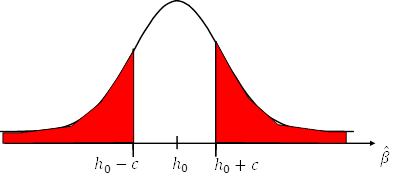
But how far is too far exactly? Or in terms of the
figure above: how big is ![]() ?
This depends on the reliability of the estimate
?
This depends on the reliability of the estimate ![]() . If we know
that the estimate is imprecise – i.e. there is a high likelihood that
. If we know
that the estimate is imprecise – i.e. there is a high likelihood that ![]() is very far
away from
is very far
away from ![]() even if H0 is
true, then we would tolerate higher values for c.
even if H0 is
true, then we would tolerate higher values for c.
With the Monte-Carlo Analysis we have seen that
·
![]() is
(approximately) normally distributed
is
(approximately) normally distributed
·
The estimate is more precise (i.e. the standard error ![]() is smaller) if
the variance of the error (
is smaller) if
the variance of the error (![]() ) is smaller or
the variance of the explanatory variable x is larger.
) is smaller or
the variance of the explanatory variable x is larger.
After running a regression it is possible to estimate ![]() (i.e. we can
label this estimate
(i.e. we can
label this estimate ![]() ) and R
provides this estimate as part of its regression output. Here is an example:
) and R
provides this estimate as part of its regression output. Here is an example:
df=read_dta("../data/foreigners.dta")
df['crimesPc']=df$crimes11/df$pop11
reg1=lm(crimesPc~b_migr11,df)
summary(reg1)
##
## Call:
## lm(formula = crimesPc ~ b_migr11, data = df)
##
## Residuals:
## Min 1Q Median 3Q Max
## -1.5886 -0.3789 -0.1038 0.2046 14.0988
##
## Coefficients:
## Estimate Std. Error t value Pr(>|t|)
## (Intercept) 0.992957 0.079387 12.508 < 2e-16 ***
## b_migr11 0.037630 0.005088 7.396 1.23e-12 ***
 ## ---
Hence, we can use the bell-shaped normal distribution (with
mean ![]() and standard
error
and standard
error ![]() ; i.e.
; i.e. ![]() ) to work out the
likelihood is for
) to work out the
likelihood is for ![]() to fall in the
rejection area even though it is true; i.e. it is the combined area under the
bell curve in the tails of the distribution for a given c.
to fall in the
rejection area even though it is true; i.e. it is the combined area under the
bell curve in the tails of the distribution for a given c.
Equally we can work out which ![]() goes along
with a given desired probability. This latter approach is what we do in
hypothesis testing. We decide first what probability (i.e. risk that we reject
the hypothesis even though it is correct) we find acceptable (e.g. 1%, 5% or
10%) and we then work out the relevant c. Those risk levels are also referred
to as significance levels.
goes along
with a given desired probability. This latter approach is what we do in
hypothesis testing. We decide first what probability (i.e. risk that we reject
the hypothesis even though it is correct) we find acceptable (e.g. 1%, 5% or
10%) and we then work out the relevant c. Those risk levels are also referred
to as significance levels.
Implementation
It turns out that instead of working out the c for a given
distribution ![]() it’s sufficient
to work out the relevant threshold numbers only once for the Standard Normal
Distribution
it’s sufficient
to work out the relevant threshold numbers only once for the Standard Normal
Distribution ![]() . The reason
for this that an estimate that is Normally distributed can always be converted
into one that is Standard Normally distributed by subtracting its expected
value and dividing by its standard error; i.e. by computing
. The reason
for this that an estimate that is Normally distributed can always be converted
into one that is Standard Normally distributed by subtracting its expected
value and dividing by its standard error; i.e. by computing
![]()
Thus, we can compare ![]() to the
thresholds for the standard normal distribution. To find those in turn we can
use the qnorm() R-function which is the inverse of the cumulative density
function. You have to provide qnorm with a probability (e.g. 0.025) and it will
tell you for which value
to the
thresholds for the standard normal distribution. To find those in turn we can
use the qnorm() R-function which is the inverse of the cumulative density
function. You have to provide qnorm with a probability (e.g. 0.025) and it will
tell you for which value ![]() the left tail
of the normal distribution will correspond to that probability
the left tail
of the normal distribution will correspond to that probability
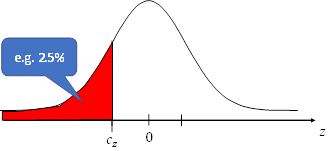
qnorm(0.025) = -1.959964
Similarly, we can find the thresholds for other possible significance levels
qnorm(0.005) = -2.575829 for 1%
qnorm(0.05) = -1.644854 for 10%
So if we find a ![]() =0.037630
(as in the example above) and
=0.037630
(as in the example above) and ![]() and we are testing the
hypothesis that
and we are testing the
hypothesis that ![]() could
be zero (H0:
could
be zero (H0: ![]() we need to
check if
we need to
check if ![]() is within the
interval implied by those values (i.e. in this case we would reject the
hypothesis even if we only allowed for a small significance level).
is within the
interval implied by those values (i.e. in this case we would reject the
hypothesis even if we only allowed for a small significance level).
What about t-statistics?
The so-called t statistic is like the z value above except that we now allow the standard error to be estimated as well:
![]()
Hence, because in practice we never know ![]() this is what we
compute in practice. As a consequence, rather than being Standard Normally distributed,
t is t distributed. Luckily this does not matter much in practice because the t
distribution is almost identical to the standard normal distribution, provided our
sample is large enough; e.g. at 12 observations the 5% threshold value would be
2.228. However, at 100 observations the threshold is -1.984467; i.e. fairly
close to the 1.96 found with the normal distribution. You can work this out
with the qt(0.025, 98) command where the second number refers to the degrees of
freedom; i.e. the number of observations minus the number of parameters in your
model (i.e. 2 in our case: intercept and slope).
this is what we
compute in practice. As a consequence, rather than being Standard Normally distributed,
t is t distributed. Luckily this does not matter much in practice because the t
distribution is almost identical to the standard normal distribution, provided our
sample is large enough; e.g. at 12 observations the 5% threshold value would be
2.228. However, at 100 observations the threshold is -1.984467; i.e. fairly
close to the 1.96 found with the normal distribution. You can work this out
with the qt(0.025, 98) command where the second number refers to the degrees of
freedom; i.e. the number of observations minus the number of parameters in your
model (i.e. 2 in our case: intercept and slope).
P-values
An even simpler way of doing the same thing (i.e. hypothesis
test) involves P values. In the past without computers this was hard but now this
is easy. P values for the hypothesis test H0: ![]() are routinely
reported along with regression output; e.g. in R it’s the values in the column Pr(>|t|).
are routinely
reported along with regression output; e.g. in R it’s the values in the column Pr(>|t|).
The P value is the significance level you would have to
choose if the value you estimated was equal to the rejection threshold; i.e. ![]() . Hence, thus
if P is very small (smaller than your desired significance level) then you
would reject the hypothesis. If it is rather large (larger than your desired
significance level) than you don’t reject your hypothesis.
. Hence, thus
if P is very small (smaller than your desired significance level) then you
would reject the hypothesis. If it is rather large (larger than your desired
significance level) than you don’t reject your hypothesis.
You can get P-values for tests other than H0: ![]() using the linearHypothesis
command (part of library(“car”)).
using the linearHypothesis
command (part of library(“car”)).
For example if you wanted to check if the migration coefficient in the example above is equal to 0.04 you could run the command
linearHypothesis(reg1, c( "b_migr11= 0.04") )
 Hypothesis:
b_migr11 = 0.04
Model 1: restricted model
Model 2: crimesPc ~ b_migr11
Res.Df RSS Df Sum of Sq F Pr(>F)
1 323 301.53
2 322 301.33 1 0.20309 0.217 0.6416